ECG Part 1: Basics
Fri Aug 07 2026
By B. Hassan

An electrocardiogram (ECG) is an easily obtained recording of the electrical activity of the heart and provides valuable information about cardiac structure and function.
Physics of a voltmeter
A voltmeter has 2 electrodes a positive and a negative electrode. A voltmeter measures the difference in electric potential between its two electrodes. The potential at each electrode is produced by the electric field generated by the entire charge distribution around the electrode. The machine then subtracts the readings from both electrodes.
When there is no difference in electric potential between the two electrodes, the voltmeter records a zero flat line.
In ECG, we assume that current flows from negative to positive such that if the positive recording electrode is at a higher electrical potential than the negative recording electrode (i.e. current moves towards the positive electrode), the recorded voltage is positive and the tracing deflects upward. If it is lower (i.e. current moves towards the negative electrode), the recorded voltage is negative and the tracing deflects downward.
Each electrode measures the electrical potential at its location, and that potential is influenced by the entire distribution of charge around the electrode, not just the charge directly beneath the electrode.
Single cell model (depolarization)
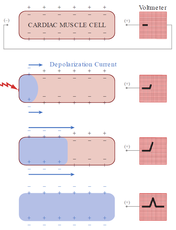
The single cell model observes the propagation of an electrical impulse along a single myocyte. We place voltmeter such that one electrode is on one side, and the other is on the opposite side of the cell.
Note
In this configuration, the voltmeter only measures the potential difference across the extracellular space, and not inside the cell. This is because the cell membrane acts as its own compartment that don’t allow charge leakage.
In the resting state, the cell is polarized; that is, the outside of the cell is electrically positive with respect to the inside as we talked about in electrophysiology of the heart. In this state, the voltmeter does not record any electrical activity, because there is no electrical potential difference between the electrodes.
This equilibrium is disturbed when the cell is stimulated, causing Na+ ions to rush into the cell, causing the polarity at the stimulated region to reverse such that the outside becomes negatively charged with respect to the inside (i.e. depolarization).
At that moment, an electrical potential is created on the cell surface between the depolarized area (negatively charged) and the still-polarized (positively charged surface) portions of the cell, causing the spread of the depolarization wave across the cell.
Because the depolarization current in this example proceeds toward the positive electrode, an upward deflection is recorded. As the depolarization wave propagates toward the positive electrode, the electrical potential difference between the two recording electrodes increases, producing an increasingly positive deflection. The potential difference reaches its maximum when the depolarization wave is approximately midway between the electrodes.
Once the cell has fully depolarized, the outside is completely negatively charged compared to the inside, the opposite of the initial resting state. However, because the surface charge is homogeneous once again, the electrodes measure a potential difference of zero and the voltmeter records a neutral “flat line” at this time.
Alternative explanation
At 25% depolarization, the negative electrode records the area around it, which contains negative charge close to the electrode and positive charge away from the electrode, while the positive electrode is influenced primarily by polarized (positive extracellular) tissue.
Then as the depolarization wave progresses up to 50%, the reading increases as the negative electrode becomes more and more exposed to negative charge while the depolarization wave hasn’t traveled far enough to affect the positive electrode.
The reading reaches its peak at 50% depolarization, when, relatively speaking, the maximum area around the positive electrode is is influenced by polarized (positive) regions and the maximum area around the negative electrode is influenced by depolarized (negative) regions.
Then at 75% depolarization, the positive reading decreases because the depolarization wave has traveled far enough to be sensed by the positive electrode. This means the area around the positive electrode contains both positive and negative charges, while the area around the negative electrode is mainly surrounded by negative charge, and so the overall electrical potential difference experienced by both electrodes decreases.
Once the cell is completely depolarized, the extracellular surface has a uniform potential. Since both electrodes now measure the same potential, the recorded voltage returns to zero.
Yet another explanation
Since electricity moves almost instantly compared to the depolarization wave, the extracellular space at partial cell depolarization can be though of as a temporary battery with a positive and a negative terminal.
Note
A small battery consisting of a positive charge and a negative charge separated by a small distance, like the one in this model is called a dipole.
When electrodes are placed on opposite terminals, they are essentially measuring the electrical potential difference across the battery terminals (i.e. the voltage of the battery).
The voltage recorded by the electrodes reaches its maximum when the depolarization wave is approximately midway between the electrodes, because this produces the greatest potential difference between the two battery terminals.
The potential difference then decreases the more the overall charge difference in the battery decreases (i.e. the more the deviation from the midpoint, whether that deviation is towards the polarized or depolarized direction).
Single cell model (repolarization)
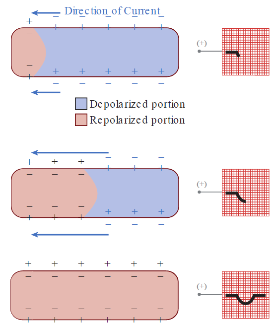
Depolarization initiates myocyte contraction and is then followed by repolarization, the process by which the cellular charges return to the resting state.
As the left side of the myocyte in our example begins to repolarize, its surface charge becomes positive once again. An electrical potential is therefore generated, and current flows from the still negatively charged surface toward the newly repolarized area. Since this current is directed away from the positive electrode, a downward defection is recorded, opposite to that which was observed during the process of depolarization.
Recall in electrophysiology of the heart that repolarization was slower than depolarization, which is why the recorded defection of repolarization is wider and of lower magnitude than that of repolarization.
ECG
So far, we have only considered the depolarization and repolarization of a single cardiac muscle cell. However, as a depolarization wave spreads through the entire heart, each cell generates electrical forces, and it is the sum of these forces measured at the surface of the skin that is recorded by an ECG machine.
It is important to note that in the intact heart, the sequence by which regions repolarize is actually opposite to that of their depolarization. This is because action potential durations are more prolonged in cells near the inner endocardium (the first cells stimulated by Purkinje fibers) than in myocytes near the outer epicardium (the last cells to depolarize). Thus, the cells close to the endocardium are the first to depolarize but are the last to repolarize. As a result, the direction of repolarization recorded by the ECG machine is usually the inverse of what was presented in the single-cell example. That is, unlike the single-cell model, the electrical defections of depolarization and repolarization in the intact heart are usually oriented in the same direction on the ECG tracing.
The direction and magnitude of the deflections on an ECG recording depend on how the generated electrical forces are aligned to a set of specific reference axes, known as ECG leads. Electrodes are placed directly on the skin, held in place by adhesive tabs, on each of the four limbs and on the chest in the standard arrangement as follows:
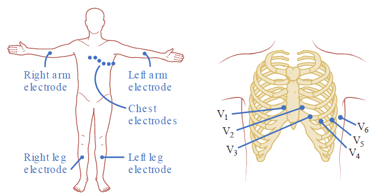
The right-leg electrode is not used for measurement but serves as an electrical ground; it acts as a reference point to eliminate ambient electrical noise that would otherwise completely drown out the heart’s tiny electrical signals.
The locations of the chest leads are:
- V1: 4th intercostal space 2 cm to the right of the sternum
- V2: 4th intercostal space 2 cm to the left of the sternum
- V3: midway between V2 and V4
- V4: 5th intercostal space, left midclavicular line
- V5: same level as V4, left anterior axillary line
- V6: same level as V4, left midaxillary line
ECG planes
A complete ECG (called a “12-lead ECG”) is produced by recording electrical activity between the electrodes in specific patterns. This results in six reference axes in the body’s frontal plane (termed limb leads) plus six in the transverse plane (termed chest leads).
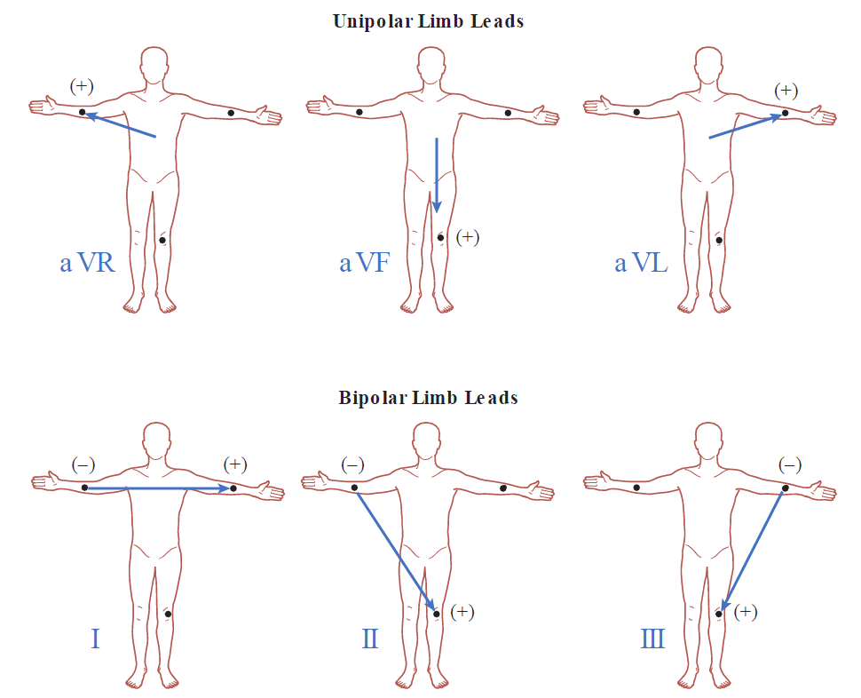
The following are the 6 limb leads. Each unipolar lead has a single positive electrode such that the negative pole is the average of the 2 other electrodes. On the other hand, each bipolar electrode has a specific designated positive and a specific negative electrode.
Note
Although these illustrations show outstretched arms, such positioning is not necessary when acquiring a patient’s ECG recording. Even when the arms are by the patient’s sides, directionality of the leads is maintained.
The aVR lead selects the the right-arm electrode as the (+) pole with respect to the other electrodes. When the electrical activity of the heart points in the direction of the right arm, an upward defection is recorded in lead aVR. Conversely, when electrical forces are directed away from the right arm, the ECG inscribes a downward deflection in aVR.
Similarly, aVF is recorded by setting the left leg as the (+) pole, such that a positive deflection is recorded when electrical activity is directed toward the feet.
Lead aVL is selected when the left-arm electrode is made the (+) pole.
In bipolar leads, the ECG machine inscribes an upward deflection if electrical forces are heading toward the (+) electrode and records a downward deflection if the forces are heading toward the (−) electrode.
A simple mnemonic to remember the bipolar leads is that the lead name indicates the number of l’s in the placement sites. For example:
- Lead I connects the left arm to the right arm
- Lead II connects the right arm to the left leg
- Lead III connects the left arm to the left leg
By overlaying these six limb leads, an axial reference system is established. The following shows that reference system. Each lead is presented with its (+) pole designated by an arrow and the (−) aspect by dashed lines. The (+) pole of lead I points to 0 degrees and by convention, measurement of the angles proceeds clockwise from 0 degrees at 30 degree increments.
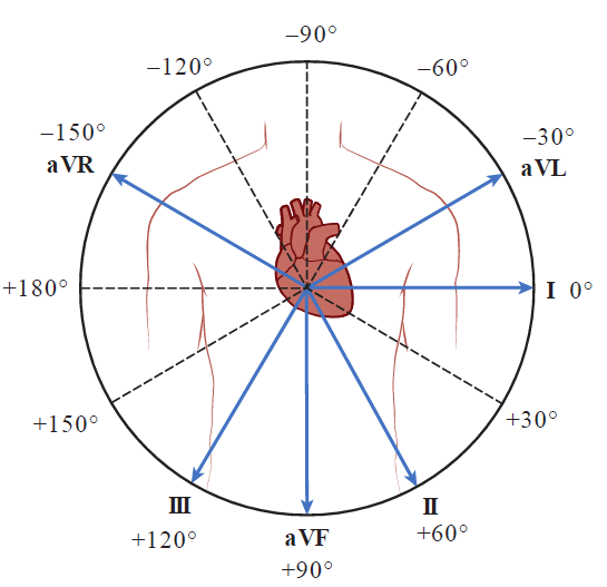
The complete ECG recording provides a simultaneous image of the heart’s electrical activity, taken from the perspective of each of these lead reference axes.
The following shows an example of depolarization waves in different directions and how they show up in lead I. Here we use lead I, but this can be applied to all leads. In image A, the direction of the electrical activity is the same as the direction of the lead, so a depolarization with a large magnitude is recorded. In image B, some component of the electrical wave vector is in a direction different to the lead, and so the magnitude recorded is smaller. Image D is similar to B except that the direction is reversed. In image C, no component in the electrical wave vector is at the direction of the lead, and so the lead records 0.
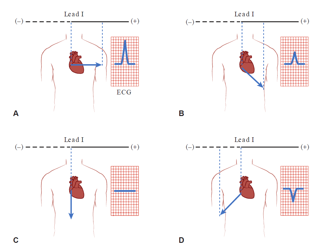
In general, the magnitude of the defection is directly proportional to how parallel the electrical force is to the axis of the lead being examined. The more parallel the electrical force is to the lead axis, the greater the magnitude of the defection.
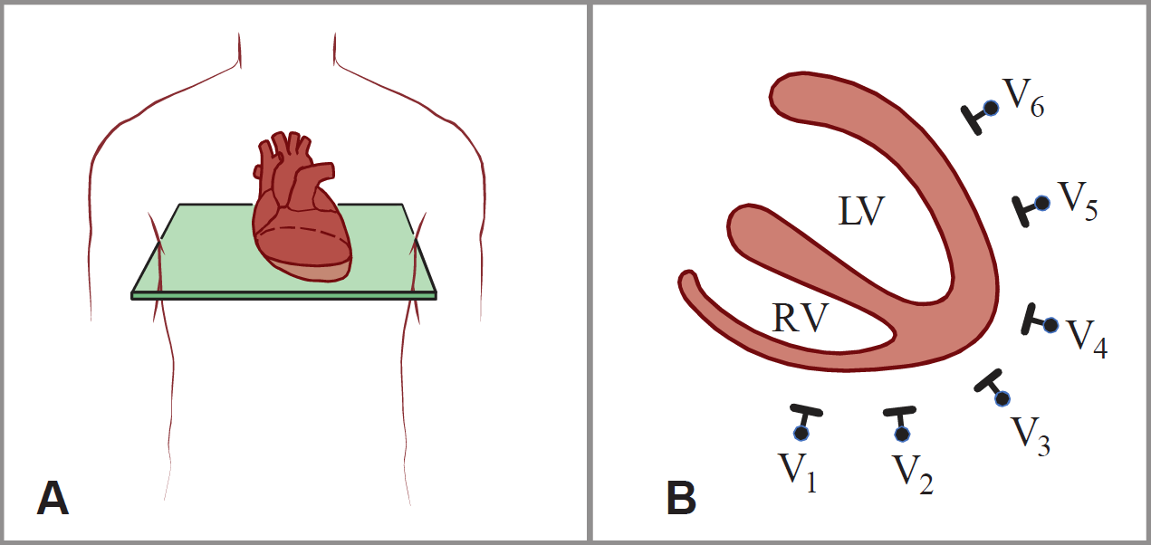
The six standard limb leads examine the electrical forces in the frontal plane of the body. However, because electrical activity travels in 3D, recordings from a perpendicular plane is also essential. This is accomplished by the use of the six electrodes placed on the chest wall creating the chest (“precordial”) leads. These are considered unipolar leads as well.
The following shows the orientation of the precordial leads with respect to the heart:
Sequence of cardiac activation
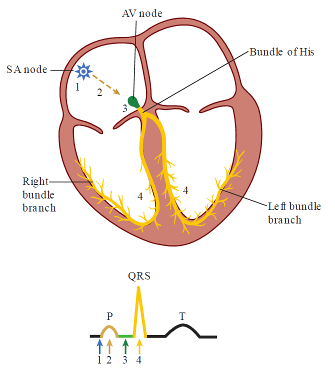
Recall that the normal beat begins at the SA node, after which the wave of depolarization spreads rapidly through the atria before reaching the AV node, where the wave of depolarization encounters a slight physiological delay. The impulse then travels rapidly through the bundle of His, dividing into right and left bundle branches. The left bundle branches divide into Purkinje fibers, which radiate throughout the myocardium.
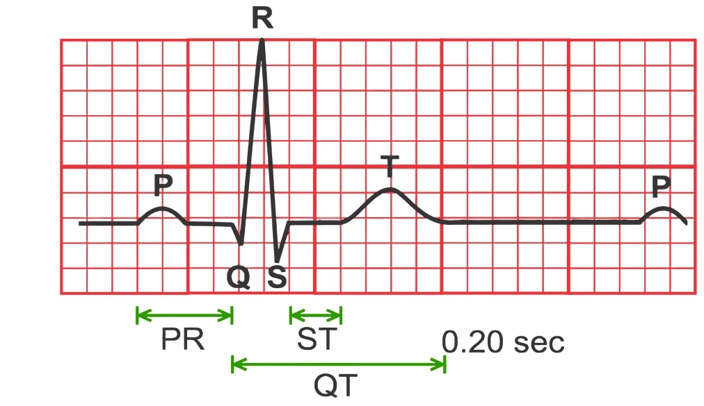
Each heartbeat is represented on the ECG by three major events that track the sequence of impulse propagation. The P wave represents depolarization of the atria. Following the P wave, the tracing returns to baseline due to the conduction delay in the AV node. After which, the ECG records the QRS complex, which represents depolarization of the ventricular muscles. After the QRS complex, the tracing returns to baseline, and after a brief delay, a T wave signals repolarization of the ventricular muscles.
In rare occasions, an additional small deflection called the U wave may follow the T wave, which is believed to represent late sequence of ventricular repolarization.
The QRS complex
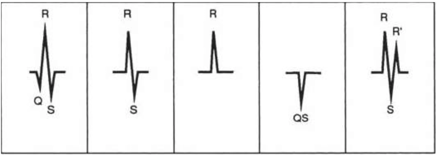
The normal QRS complex may take one of several shapes but can always be subdivided into individual components. The first deflection of the QRS complex is known as the Q wave, and is a downward deflection.
If the first defection in the QRS complex is upward, then that particular QRS complex does not have a Q wave.
The R wave is defined as the first upward defection within the QRS complex, whether or not a Q wave is present. Any downward deflection following the R wave is known as an S wave.
The following shows several common variations of the QRS complex. In certain pathologic states, additional deflections may be inscribed:
The following shows the course of normal ventricular depolarization as it is recorded in the frontal plane by the aVF and aVL leads. The recording in aVF represents electrical activity from the perspective of the inferior aspect of the heart and aVL records from the perspective of the left lateral side.
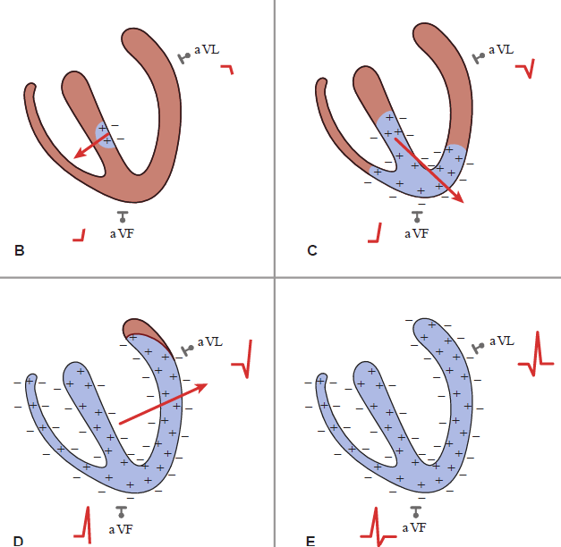
The initial portion of ventricular myocardium that is depolarized with a given cardiac cycle is the midportion of the interventricular septum. Because depolarization reverses the cellular charge, the surface of that region becomes negative with respect to the inside. The initial current is directed toward the right ventricle and inferiorly. Because the force is directed away from the positive pole of the aVL lead, an initial downward deflection is recorded by that lead. At the same time, the electrical impulse is directed toward the positive pole region of the aVF lead, causing an upward deflection to be recorded there.
As the lateral walls of the ventricles are depolarized, the electrical impulse of the thicker left side far outweigh that of the right. Therefore, the arrow’s orientation is increasingly directed toward the left ventricle. At complete depolarization, the myocytes are again homogeneously charged, thus no further net electrical force is generated, and the ECG recording returns to baseline in both leads.
The sequence of ventricular depolarization can similarly be examined in the transverse plane from the precordial leads. Because the initial forces are directed anteriorly (i.e. toward the positive pole of V1), the initial defection recorded by lead V1 is upward. These same initial forces are directed away from V6, so an initial downward defection is recorded there.
As the wave of depolarization spreads, the electrical impulses of the left ventricle outweigh those of the right, and the vector swings posteriorly toward the bulk of the left ventricle. As the forces swing away from lead V1, the deflection there becomes downward, whereas it becomes more upright in lead V6. Leads V2 through V5 record intermediate steps in this process, such that the R wave becomes progressively taller from lead V1 through lead V6, a pattern known as “R-wave progression.”
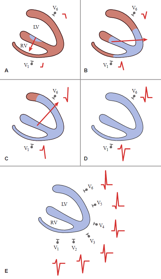
Typically, the height of the R wave becomes greater than the depth of the S wave in lead V3 or V4; the lead in which this occurs is termed the “transition” lead. In this example, V4 is the transition lead.
Clinical interpretation of the ECG
The ECG tracing is recorded on a special grid dividing into thinner and thicker lines. The distance between each thin line is 1mm in both the horizontal and the vertical directions. Each fifth line in both the horizontal and vertical directions is a thick line.
The y-axis (vertical axis) tracks the voltage in millivolts (mV) such that each 1mm vertical line represents 0.1 mV, and each thick line (5mm) represents 0.5 mV.
The x-axis (horizontal axis) tracks time such that each 1mm division represents 0.04 seconds and each thick line (5mm) represents 0.2 seconds.
When describing an ECG tracing, a commonly followed sequence of an analysis is:
- Check voltage calibration
- Heart rhythm
- Heart rate
- Intervals (PR, QRS, QT)
- Mean QRS axis
- Abnormalities of the P wave
- Abnormalities of the QRS (hypertrophy, bundle branch block, infarction)
- Abnormalities of the ST segment and T wave
Calibration
ECG machines routinely inscribe a 1.0-mV vertical signal at the beginning or end of each tracing to document the voltage calibration of the machine. In the normal case (i.e. when each 1-mm vertical box represents 0.1 mV), that calibration signal is 1cm, and so is recorded on 2 large boxes.
However, in patients with markedly increased voltage of the QRS complex, the very large deflections do not fit on the standard tracing. To facilitate interpretation in such a case, the recording is often purposely made at half the standard voltage (i.e., each 1-mm box = 0.2 mV), and this is indicated on the ECG tracing by a change in the height of the 1.0-mV calibration signal. For example, at half the standard voltage, the signal would be 5mm tall, or only 1 large box.
Heart rhythm
The normal cardiac rhythm initiated by the sinus node, is known as the sinus rhythm. An ECG tracing shows sinus rhythm if all of the following criteria are met:
-
There is a one-to-one relationship between P and QRS waves meaning that each P wave must be followed by a QRS complex, and each QRS complex must be preceded by a P wave.
-
The P wave is upright in leads I, II, and aVF, and inverted in aVR
-
The PR interval must be between 0.12 and 0.20 seconds (3 to 5 small boxes).
These conditions actually make sense if you stop and think about it. Condition 1 ensures that the impulse generated by the SA node actually reaches the ventricles, producing a corresponding ventricular depolarization.
As for condition 2, it says that the impulse generated by the SA node must move in the directions of leads I, II, and aVF. Looking at the directions of these leads, this condition says that the signal must be moving towards the left atrium and towards the AV node. In other words, this condition ensures that the impulse generated by the SA node is moving in the correct direction and is propagating correctly.
Condition 3 is another way of expressing the normal impulse delay that occurs in the AV node.
Heart rate
The heart rate can be calculated from an ECG using the following equation:
When it is not necessary to determine the exact heart rate, a simple memorized technique that is routinely used is to count the number of large boxes between two consecutive QRS complexes, using the sequence:
For example, if there are 3 large boxes between two consecutive QRS complexes, then the heart rate is approximately 100 bpm.
If the heart rate is regular sinus rhythm, then:
-
If the heart rate is between 60 and 100 bpm, then this is called normal sinus rhythm.
-
If the heart rate is less than 60 bpm, then this is called sinus bradycardia.
-
If the heart rate is greater than 100 bpm, then this is called sinus tachycardia.
When the rhythm is irregular, these estimates cannot be easily applied, so the heart rate in such cases may be better approximated by counting the number of QRS complexes during 6 seconds of the trace and multiplying that number by 10. ECG tracings usually have time markers, spaced 3 seconds apart printed at the top or bottom of the tracing that facilitates this calculation.
Intervals
-
The PR interval is measured from the start of the P wave to the start of the QRS complex
-
The QRS interval is measured from the start to the end of the QRS complex
-
The QT interval is measured from the beginning of the QRS complex to the end of the T wave
These intervals are shown in the following image:
For each of these, it is appropriate to take the measurement in the lead in which the interval is the longest in duration.
Because the QT interval varies with heart rate (the faster the heart rate, the shorter the QT), the corrected QT (QTc) interval is determined by dividing the measured QT interval by the square root of the RR interval.
When the heart rate is in the normal range (60-100 bpm), a rapid rule can be applied: if the QT interval is visually less than half the RR interval, then the QT interval is within the normal range.
The normal ranges for each interval are:
- PR interval: 0.12–0.20 sec (3–5 small boxes)
- QRS interval: sec ( small boxes)
- Corrected QT: sec
Mean QRS Axis
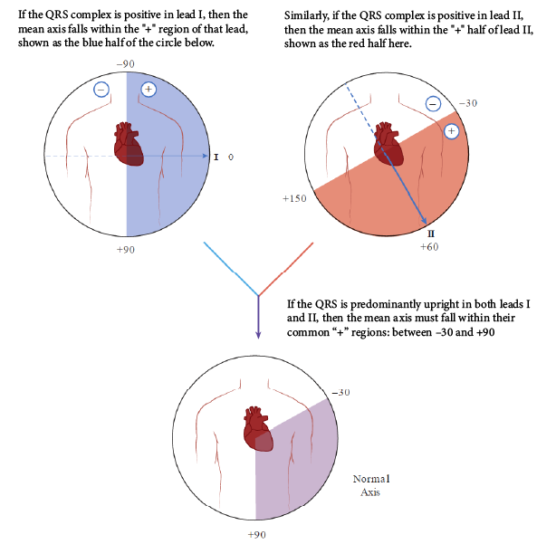
The mean QRS axis represents the average of the electrical waves generated during the sequence of ventricular depolarization as measured in the frontal plane. The normal value is between −30 degrees and +90 degrees.
A mean axis more negative than −30 degrees implies left axis deviation, whereas an axis greater than +90 degrees implies right axis deviation.
To determine whether the axis is normal or abnormal, examine the QRS complexes in leads I and II. If the QRS is primarily positive in both leads (i.e. the upward deflection is greater than the downward deflection), then the mean vector falls within the normal range and no further calculation is necessary. However, if the QRS in either lead is not primarily upward, then the axis is abnormal, and the approximate axis should then be determined by one of the following more precise methods.
Note
Some resources may recommend examining leads I and aVF to determine whether the mean axis falls in the normal range. However, this may produce errors in certain cases, and so it is recommended to examine leads I and II instead.
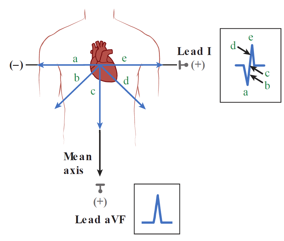
In order to determine the mean axis with greater precision when necessary, we have to first understand what an isoelectric QRS complex is. An isoelectric QRS complex refers to a QRS complex where the upward positive deflections are equal in size to the downward negative deflections.
When a limb lead inscribes an isoelectric QRS complex, it indicates that the mean electrical axis of the ventricles is perpendicular to that lead. Therefore, an easy way to determine the mean QRS axis is to glance at the six limb lead recordings and observe which one has the most isoelectric-appearing QRS complex: the mean axis is simply perpendicular to it.
However, when the mean axis is perpendicular to a lead, it could be perpendicular in either a clockwise or a counterclockwise direction. Determining which of these is correct requires inspecting the recording of the lead that is perpendicular to the one inscribing the isoelectric complex (and is therefore parallel to the mean axis). If the QRS is predominantly upright in that perpendicular lead, then the mean vector points toward the (+) pole of that lead. If it is predominantly negative, then it points away from the lead’s (+) pole.
Consider the following example. Lead I shows an isoelectric QRS complex, so the mean axis must be perpendicular to lead I. But there are 2 directions that are perpendicular to lead I, one is at and the other at . So we look at lead aVF, which is the lead perpendicular to lead I. Here we see that the QRS complex in the lead is purely positive, and so the mean axis must be towards the aVF lead.
To summarize, the mean QRS axis is calculated as follows:
-
Inspect leads I and II. If the QRS is primarily upward in both, then the axis is normal and you are done. If not, proceed to step 2.
-
Inspect the six limb leads and determine which one contains the QRS that is most isoelectric. The mean axis is perpendicular to that lead.
-
Inspect the lead that is perpendicular to the lead containing the isoelectric complex. If the QRS in that perpendicular lead is primarily upward, then the mean axis points to the positive pole of that lead. If primarily negative, then the mean axis points to the negative pole of that lead.
In some patients, isoelectric complexes are inscribed in all the limb leads. This happens when the heart is tilted such that the mean QRS axis points straight forward or back from the frontal plane, as may be the case in patients with chronic obstructive lung disease; in such cases, the mean axis is said to be indeterminate.
Abnormalities of the P Wave
The P wave represents depolarization of the right atrium followed quickly by the depolarization of the left atrium, with the two components being nearly superimposed. The P wave is usually best visualized in lead II, the lead that is most parallel to the flow of electrical current through the atria from the SA to the AV nodes.
When the right atrium is enlarged, the initial component of the P wave is larger than normal (the P is taller than 2.5 mm in lead II).
Left atrial enlargement is best observed in lead V1. Normally, V1 inscribes a P wave with an initial positive deflection reflecting right atrial depolarization, followed by a negative deflection, owing to the left atrial forces oriented posteriorly. Left atrial enlargement therefore manifests by a greater than normal negative defection (at least 1 mm wide and 1 mm deep) in lead V1.